Saving Array Quantities

Overview

Questions

• How can I save per-particle quantities for later analysis?

• How can I access that data?

Objectives

• Show how to log per-particle properties to a GSD file.

• Explain how to read logged quantities from a GSD file.

• Mention that OVITO reads these quantities.

Boilerplate code

import gsd.hoomd
import hoomd
import matplotlib
import numpy

%matplotlib inline
matplotlib.style.use('ggplot')
import matplotlib_inline

matplotlib_inline.backend_inline.set_matplotlib_formats('svg')

The render function in the next (hidden) cell will render the system state using fresnel. Find the source in the hoomd-examples repository.

General array quantities

You logged scalar and array quantities to a HDF5 file in the previous section. HDF5 is the ideal format to log this type of data, as it produces small files that can be read quickly.

Array quantities coupled with a trajectory

You can also log scalar, array, per-particle (e.g. energy and force), and other quantities in a GSD file along with the trajectory. Then you can use utilize the data in your analysis and visualization workflow, such as using OVITO to color particles by energy or display force vectors. When using OVITO, open the GSD file and all logged quantities will be available in the inspector and for use in the pipeline.

Define the Simulation

This tutorial executes the Lennard-Jones particle simulation from a previous tutorial. See Introducing Molecular Dyamics for a complete description of this code.

cpu = hoomd.device.CPU()
simulation = hoomd.Simulation(device=cpu, seed=1)
simulation.create_state_from_gsd(
    filename='../01-Introducing-Molecular-Dynamics/random.gsd'
)

integrator = hoomd.md.Integrator(dt=0.005)
cell = hoomd.md.nlist.Cell(buffer=0.4)
lj = hoomd.md.pair.LJ(nlist=cell)
lj.params[('A', 'A')] = dict(epsilon=1, sigma=1)
lj.r_cut[('A', 'A')] = 2.5
integrator.forces.append(lj)
nvt = hoomd.md.methods.ConstantVolume(
    filter=hoomd.filter.All(), thermostat=hoomd.md.methods.thermostats.Bussi(kT=1.5)
)
integrator.methods.append(nvt)
simulation.operations.integrator = integrator
simulation.run(0)

Logging per-particle quantities

MD forces provide a number of loggable quantities including their contribution to the system energy, but also per-particle energy contributions (in energies) and per-particle forces, torques, and virials.

lj.loggables

{'energy': 'scalar',
 'energies': 'particle',
 'additional_energy': 'scalar',
 'forces': 'particle',
 'torques': 'particle',
 'virials': 'particle',
 'additional_virial': 'sequence'}

Add the per-particle LJ energies and forces to a logger:

logger = hoomd.logging.Logger()
logger.add(lj, quantities=['energies', 'forces'])

Writing per-particle quantities to a GSD file

Create the GSD writer to write the simulation trajectory:

gsd_writer = hoomd.write.GSD(
    filename='trajectory.gsd',
    trigger=hoomd.trigger.Periodic(10000),
    mode='xb',
    filter=hoomd.filter.All(),
)
simulation.operations.writers.append(gsd_writer)

Set the logger attribute and GSD will also store the selected quantities.

gsd_writer.logger = logger

Run the simulation:

simulation.run(100000)

Flush the GSD buffer so it is readable in the next code cell. In typical workflows, you will run separate simulation and analysis scripts and the buffered writes will automatically flush when your simulation script exits.

gsd_writer.flush()

Reading logged data from a GSD file

Use the gsd package to open the file:

traj = gsd.hoomd.open('trajectory.gsd', mode='r')

The log data for a specific frame is stored in the log dictionary for that frame.

traj[0].log.keys()

dict_keys(['particles/md/pair/LJ/energies', 'particles/md/pair/LJ/forces'])

GSD prepends particles/ to the logged name of per-particle quantities. The quantities are NumPy arrays with N_particles elements. Here are a few slices:

traj[-1].log['particles/md/pair/LJ/energies'][0:10]

array([-2.48199661, -2.12335126, -4.00387093, -2.63144287, -2.18554869,
       -2.32050608, -2.02647941, -2.44569987, -2.53925901, -2.40447241])

traj[-1].log['particles/md/pair/LJ/forces'][0:10]

array([[ -2.79783236,  -1.1447838 ,  -2.29953834],
       [  1.34913891,   2.73176148,  -2.13988326],
       [  3.18757211, -12.6700367 ,  -1.80576571],
       [ -4.70877614,   3.40071066,  -8.78080297],
       [  4.94235545,   6.16337821,  -6.97153234],
       [ -3.2043855 ,   0.18160722,  -1.14755586],
       [-10.73489983,   0.28556186,   4.2747685 ],
       [ -2.20080722,  -1.70941385,  16.53612282],
       [  4.01219479,   1.53498589,   3.94355533],
       [  2.1649503 ,   1.18676842,  -6.51449987]])

You can use these arrays as inputs to any computation or plotting tools:

numpy.mean(traj[-1].log['particles/md/pair/LJ/forces'], axis=0)

array([ 5.03069808e-17,  1.64798730e-16, -2.04697370e-16])

fig = matplotlib.figure.Figure(figsize=(5, 3.09))
ax = fig.add_subplot()
ax.hist(traj[-1].log['particles/md/pair/LJ/energies'], 100)
ax.set_xlabel('potential energy')
ax.set_ylabel('count')
fig

As with scalar quantities, the array quantities are stored separately in each frame. Use a loop to access a range of frames and compute time-series data or averages.

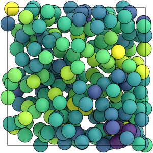
This is what the system looks like when you color the particles by the values in particles/md/pair/LJ/energies:

render(traj[-1])

In this section, you have logged per-particle quantities to a GSD file during a simulation run and accessed that data with a script. The next section of this tutorial demonstrates how to log particle shape information that OVITO can use.