Initializing the System State
Overview
Questions
How do I place particles in the initial condition?
What units does HOOMD-blue use?
Objectives
Describe the basic properties of the initial condition, including particle position, orientation, type and the periodic box.
Briefly describe HOOMD-blue’s system of units.
Demonstrate writing a system to a GSD file.
Show how to initialize Simulation state from a GSD file.
Boilerplate Code
[1]:
import itertools
import math

import hoomd
import numpy
The render function in the next (hidden) cell will render the initial condition using fresnel. Find the source in the hoomd-examples repository.
Components of the System State
You need to initialize the system state before you can run a simulation. The initial condition describes the position and orientation of every particle in the system and the periodic box at the start of the simulation.
The hard regular octahedra system self-assembles the bcc structure. Self-assembly is a process where particles will organize themselves into an ordered structure at equilibrium. Most self-assembly studies run simulations of many thousands of particles for tens of hours. To keep this tutorial short, it simulations a small number of particles commensurate with the bcc structure (2 * m**3, where m is an integer).
[4]:
m = 4
N_particles = 2 * m**3
Placing Particles
In hard particle Monte Carlo, valid particle configurations have no overlaps. The octahedron particle in this tutorial sits inside a sphere of diameter 1, so place particles a little bit further than that apart on a KxKxK simple cubic lattice of width L. The following sections of this tutorial will demonstrate how to randomize this ordered configuration and compress it to a higher density.
[5]:
spacing = 1.2
K = math.ceil(N_particles ** (1 / 3))
L = K * spacing
In HOOMD, particle positions must be placed inside a periodic box. Cubic boxes range from -L/2 to L/2. Use itertools and numpy to place the positions on the lattice in this range.
[6]:
x = numpy.linspace(-L / 2, L / 2, K, endpoint=False)
position = list(itertools.product(x, repeat=3))
print(position[0:4])
[(np.float64(-3.5999999999999996), np.float64(-3.5999999999999996), np.float64(-3.5999999999999996)), (np.float64(-3.5999999999999996), np.float64(-3.5999999999999996), np.float64(-2.3999999999999995)), (np.float64(-3.5999999999999996), np.float64(-3.5999999999999996), np.float64(-1.1999999999999997)), (np.float64(-3.5999999999999996), np.float64(-3.5999999999999996), np.float64(0.0))]
Filter this list down to N particles because K*K*K >= N_particles .
[7]:
position = position[0:N_particles]
You also need to set the orientation for each particle. HOOMD represents orientations with quaternions. The quaternion (1, 0, 0, 0) represents no rotation. Set that for all particles:
[8]:
orientation = [(1, 0, 0, 0)] * N_particles
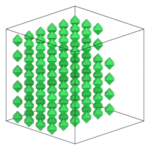
Here is what the system looks like now:
[9]:
render(position, orientation, L)
[9]:
Units
HOOMD-blue does not adopt any particular real system of units. Instead, HOOMD-blue uses an internally self-consistent system of units and is compatible with many systems of units. For example: if you select the units of meter, Joule, and kilogram for length, energy and mass then the units of force will be Newtons and velocity will be meters/second. A popular system of units for nano-scale systems is nanometers, kilojoules/mol, and atomic mass units.
In HPMC, the primary unit is that of length. Mass exists, but is factored out of the partition function and does not enter into the simulation. The scale of energy is irrelevant in athermal HPMC systems where overlapping energies are infinite and valid configurations have zero potential energy. However, energy does appear implicitly in derived units like . In HPMC, defaults to 1 energy. You can convert a pressure in HPMC’s units to a non-dimensional value with where is a representative length in your system, such as the particle’s diameter or edge length.
Writing the Configuration to the File System
GSD files store the periodic box, particle positions, orientations, and other properties of the state. Use the GSD Python package to write this file.
[10]:
import gsd.hoomd
The Frame object stores the state of the system.
[11]:
frame = gsd.hoomd.Frame()
frame.particles.N = N_particles
frame.particles.position = position
frame.particles.orientation = orientation
Each particle also has a type. In HPMC, each type has its own shape parameters. There is a single type in this tutorial, so set a type id of 0 for all particles (type ids are 0-indexed):
[12]:
frame.particles.typeid = [0] * N_particles
Every particle type needs a name. Names can be any string. HOOMD-blue uses the type names to match the parameters you specify in operations with the type names present in the state. Give the name 'octahedron' to the type id 0:
[13]:
frame.particles.types = ["octahedron"]
GSD represents boxes with a 6-element array. Three box lengths L_x, L_y, L_z, and 3 tilt factors. Set equal box lengths and 0 tilt factors to define a cubic box.
[14]:
frame.configuration.box = [L, L, L, 0, 0, 0]
Write this snapshot to lattice.gsd:
[15]:
with gsd.hoomd.open(name="lattice.gsd", mode="x") as f:
    f.append(frame)
Initializing a Simulation
You can use the file to initialize the Simulation state. First, create a Simulation:
[16]:
cpu = hoomd.device.CPU()
simulation = hoomd.Simulation(device=cpu)
Then use the create_state_from_gsd factory function to read in the GSD file and populate the state with the particles and box from the file:
[17]:
simulation.create_state_from_gsd(filename="lattice.gsd")
The next section in this tutorial will show you how to use HPMC to randomize the particle positions and orientations.