Active Brownian Particle Systems

Overview

Questions

• How can we model particles with self-induced active forces?

Objectives

• Write an MD simulation for spherical active particles using the Active Brownian Particle (ABP) model.

• Learn how to implement a simulation with the OverdampedViscous method and rotational diffusion to initialize and thermalize an active particle system that we can then visualize.

Boilerplate Code

import itertools

import gsd.hoomd
import hoomd
import numpy

The render function in the next (hidden) cell will render a snapshot using fresnel. Find the source in the hoomd-examples repository.

Simulating Brownian Active Particles

In this part of the tutorial, we will create a simulation of self-propelled active particles using the Active Brownian Particle (ABP) model.

Péclet number and activity

Activity drives persistent motion that breaks equilibrium detailed balance and is typically quantified by the Péclet number (Pe). This is a key dimensionless parameter in active matter that quantifies the relative strength of persistent active motion versus random thermal diffusion. For spherical ABPs in 2D this is typically defined as $Pe = v_0 \cdot \sigma / D_{r}$ where

• $v_{0}$ = self-propulsion speed (active force per friction)

• $\sigma$ = particle diameter (typically = 1 in reduced units)

• and $D_{r}$ = rotational diffusion coefficient

In HOOMD-blue, the propulsion velocity is controlled by applying an active force to particles in the system. The relationship between these quantities is $v_{0} = F_{active} / \gamma$ where $\gamma$ is the translational drag coefficient (often we set $\gamma$ = 1 in overdamped Brownian dynamics). $D_{r}$ is typically set directly in the integrator as rotational diffusion. Thus we can define Pe:

$$Pe = \frac{F_{active} \cdot \sigma}{D_{r} \cdot \gamma}$$

Higher activity can induce clustering even at densities too low for passive phase separation. This phenonmenon is called motility-induced phase separation (MIPS) and will be discussed in the following section of this tutorial series.

Active Brownian Particles

Active Brownian Particles (ABPs) are among the most widely studied minimal models of active matter. They describe self-propelled particles moving in a noisy environment, where inertia is negligible and fluctuations play an essential role. For example, consider the Janus particle described earlier. The self-propulsion vector points along the axis of asymmetry, while collisions with solvent molecules lead to gradual random reorientation.

Changes in the effective temperature can alter the amount of stochastic movement experienced by the particles. In HOOMD-blue, we can model ABPs by adding a persistent self-propulsion force of fixed magnitude directed along the orientation vector. Thermal noise can enter the model through an integrator and controls the strength of both rotational and translational fluctuations. Rotational diffusion introduces noise to the orientation of the propulsion direction, causing the particle’s orientation to decorrelate over time and randomize the long-time trajectory. In HOOMD-blue typical choices of integrators include the Brownian or OverdampedViscous methods.

We can set up the initial state of the simulation in a very similar manner to previous methods we have used in earlier hoomd MD simulation tutorials.

Set up the Simulation

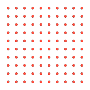
We will first initialize a system of spherical particles with a given particle density in an array. We save an initial snapshot of the current state of the system.

rho = 0.3  # particle area density
simseed = 1

m = 10
N_particles = m**2
K = numpy.ceil(N_particles ** (1 / 2))
L = (N_particles / rho) ** (1 / 2)
spacing = L / K
x = numpy.linspace(-L / 2, L / 2, int(K), endpoint=False)

position_2D = numpy.array(list(itertools.product(x, repeat=2))) + [
    spacing / 2,
    spacing / 2,
]
position_3D = numpy.hstack([position_2D, numpy.zeros((N_particles, 1))])

frame = gsd.hoomd.Frame()
frame.particles.N = N_particles
frame.particles.position = position_3D
frame.particles.typeid = [0] * N_particles
frame.configuration.box = [L, L, 0, 0, 0, 0]
frame.particles.types = ["A"]
frame.particles.mass = [1] * N_particles

# randomized orientations
rng = numpy.random.default_rng()
theta = rng.uniform(0, 2 * numpy.pi, N_particles)

frame.particles.orientation = numpy.column_stack(
    (
        numpy.cos(theta / 2),  # w
        numpy.zeros(N_particles),  # x
        numpy.zeros(N_particles),  # y
        numpy.sin(theta / 2),  # z
    )
)

with gsd.hoomd.open(name="lattice.gsd", mode="w") as f:
    f.append(frame)

Configure this simulation to run on CPU from this snapshot as we have in previous tutorials. We confirm that the box is correctly set to simulate in 2D by checking if hoomd.Box.is2D is True.

cpu = hoomd.device.CPU()
sim = hoomd.Simulation(device=cpu, seed=simseed)
state = sim.create_state_from_gsd(filename="lattice.gsd")

if hoomd.Box.is2D:
    print("True. Lz = 0 in the simulation box.")

render(sim.state.get_snapshot())

True. Lz = 0 in the simulation box.

Defining Interactions in an Active Particle system

This simulation uses the OverdampedViscous dynamics method with a drag force set by gamma. More documentation on the method OverdampedViscous can be found in the HOOMD documentation.

Add this method to our integrator.

gamma = 1

filter_all = hoomd.filter.All()
overdamped = hoomd.md.methods.OverdampedViscous(filter=filter_all)
overdamped.gamma.default = gamma

integrator = hoomd.md.Integrator(dt=0.001, integrate_rotational_dof=False)
sim.operations.integrator = integrator
integrator.methods.append(overdamped)

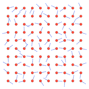
Below, hoomd.md.force.Active is the HOOMD class used to create an active force object. active.active_force["A"] specifies the components of the active force for particles of type “A” in the particle’s body frame. The Active force class also requires an active torque to be specified through active.active_torque. Here, we set this torque to zero. The active force object is then added to the integrator so that it is included in the force calculation at every timestep.

Next, we create a rotational_diffusion_updater, which applies rotational Brownian diffusion to each particle’s orientation at every timestep. As a result, each particle gradually loses memory of its initial orientation, causing the propulsion direction to evolve over time. Without this updater, particle orientations would remain fixed, so each particle would continue swimming indefinitely in a straight line. This would correspond to active ballistic motion, whereas including rotational diffusion produces the ABP dynamics that we aim to model here.

Below we set our active_force = 0.3 ($F_{\text{active}}$) and rotational_diffusion = 0.1 ($D_{r}$). Since, we have previously set gamma=1 and sigma=1 our Péclet number is 3 according to the relation defined above.

activity = 0.3
rotational_diffusion = 0.1

active = hoomd.md.force.Active(filter=filter_all)
active.active_force["A"] = (activity, 0, 0)
active.active_torque["A"] = (0, 0, 0)

integrator.forces.append(active)

rotational_diffusion_updater = active.create_diffusion_updater(
    trigger=1, rotational_diffusion=0.1
)
sim.operations += rotational_diffusion_updater

Run the simulation and get an early snapshot.

logger = hoomd.logging.Logger(["particle", "constraint"])
gsd_oper = hoomd.write.GSD(
    trigger=hoomd.trigger.Periodic(100),
    filename="active.gsd",
    logger=logger,
    mode="wb",
    dynamic=["momentum", "property"],
    filter=filter_all,
)

sim.operations += gsd_oper

sim.run(1)
render(sim.state.get_snapshot())

Run the simulation.

sim.run(10000)
render(sim.state.get_snapshot())

In this tutorial, we have successfully placed active self-propelled particles in a non-equilibrium MD simulation.

In the next tutorial, we will explore a 2D system of purely repulsive active particles that exhibit gas-liquid coexistence at intermediate densities. As briefly mentioned above, this phenomenon is known as motility-induced phase separation (MIPS).