Running Rigid Body Simulations

Overview

Questions

• How do I initialize rigid bodies from a GSD file?

• How do I integrate the rigid bodies in my simulation?

• How are thermodynamic quantities of rigid bodies measured?

Objectives

• Describe how to continue simulations from a GSD file.

• Explain integration of rotational degrees of freedom.

• Show how to exclude intra-body pairwise interactions.

• Run a rigid body MD simulation at constant temperature.

• Demonstrate that rigid bodies equilibrate both translational and rotational degrees of freedom.

Boilerplate code

import math

import hoomd

The render function in the next (hidden) cell will render the system state using fresnel.

This is not intended as a full tutorial on fresnel - see the fresnel user documentation if you would like to learn more.

Continuing the simulation from a GSD file.

The previous section created an initial condition containing dimer particles in lattice.gsd. Initialize a new simulation from this file:

cpu = hoomd.device.CPU()
sim = hoomd.Simulation(device=cpu, seed=1)
sim.create_state_from_gsd(filename='lattice.gsd')

hoomd.md.constrain.Rigid is responsible for applying the rigid body constraints to the particles in the simulation.

Create the rigid constraint:

rigid = hoomd.md.constrain.Rigid()

The body property of Rigid is not saved to the GSD file. You need to define the parameters again in the new simulation:

rigid.body['dimer'] = {
    "constituent_types": ['A', 'A'],
    "positions": [[-1.2, 0, 0], [1.2, 0, 0]],
    "orientations": [(1.0, 0.0, 0.0, 0.0), (1.0, 0.0, 0.0, 0.0)],
    "charges": [0.0, 0.0],
    "diameters": [1.0, 1.0]
}

In workflows, you can store this in a file of your choosing or use the project document in signac.

Integrating rigid body degrees of freedom

Create an Integrator with the option integrate_rotational_dof=True:

integrator = hoomd.md.Integrator(dt=0.005, integrate_rotational_dof=True)
sim.operations.integrator = integrator

The default value of integrate_rotational_dof is False, When False, the integrator will ignore all torques on particles and integrate only the translational degrees of freedom. When True, the integrator will integrate both the translational and rotational degrees of freedom.

Assign the rigid constraint to the integrator’s rigid attribute to apply the constraints during the simulation.

integrator.rigid = rigid

The translational and rotational degrees of freedom are given to the central particles of the rigid bodies. Select only the rigid centers and free particles for the integration method:

kT = 1.5
rigid_centers_and_free = hoomd.filter.Rigid(("center", "free"))
nvt = hoomd.md.methods.NVT(kT=kT, tau=1., filter=rigid_centers_and_free)
integrator.methods.append(nvt)

Defining Pair Potentials Between Bodies

Create a neighbor list with body exclusions so that the pair potential does not compute intra-body interactions:

cell = hoomd.md.nlist.Cell(buffer=0, exclusions=['body'])

Without body exclusions, the simulation may be numerically unstable due to round-off errors when subtracting large numbers. In either case, the intra-body forces contribute 0 to the net force and 0 to the net torque, so there is no need to compute them.

Apply the Lennard-Jones potential between A-A particle pairs.

lj = hoomd.md.pair.LJ(nlist=cell)
lj.params[('A', 'A')] = dict(epsilon=1, sigma=1)
lj.r_cut[('A', 'A')] = 2.5

The central particles (type dimer) are also present in the system. Make the dimer particles non-interacting with a 0 r_cut:

lj.params[('dimer', ['dimer', 'A'])] = dict(epsilon=0, sigma=0)
lj.r_cut[('dimer', ['dimer', 'A'])] = 0

You do not have to make the central particles non-interacting. You can choose any potential parameters suitable for your model.

integrator.forces.append(lj)

Compressing the system

We have initialized the system state, added the integrator, set the rigid constraint, and defined the pairwise particle interactions. Before we run the simulation, we need to set initial velocities and angular momenta of the rigid body central particles and free particles:

sim.state.thermalize_particle_momenta(filter=rigid_centers_and_free, kT=kT)
sim.run(0)
nvt.thermalize_thermostat_dof()

thermalize_particle_momenta assigns gaussian distributed momenta to each translational and rotational degree of freedom for each particle given in the filter. In this case, it wil assign momenta about the y and z axes, but not x because \(I_{xx} = 0\).

Now we can run the simulation to randomize the body positions and orientations:

sim.run(1000)

render(sim.state.get_snapshot())

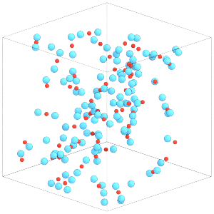
This simulation box is dilute. Compress the box to a higher density state before continuing:

initial_box = sim.state.box
final_box = hoomd.Box.from_box(initial_box)  # make a copy of initial_box
final_box.volume = initial_box.volume / 16
box_resize_trigger = hoomd.trigger.Periodic(10)
ramp = hoomd.variant.Ramp(A=0, B=1, t_start=sim.timestep, t_ramp=20000)
box_resize = hoomd.update.BoxResize(box1=initial_box,
                                    box2=final_box,
                                    variant=ramp,
                                    trigger=box_resize_trigger)
sim.operations.updaters.append(box_resize)

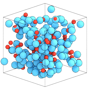
Run the simulation to compress the box:

sim.run(30000)

render(sim.state.get_snapshot())

Thermodynamic properties of rigid bodies

Add the ThermodynamicQuantities compute to the simulation:

thermodynamic_quantities = hoomd.md.compute.ThermodynamicQuantities(
    filter=hoomd.filter.All())

sim.operations.computes.append(thermodynamic_quantities)

ThermodynamicQuantities computes translational and rotational kinetic energy separately:

thermodynamic_quantities.translational_kinetic_energy

136.95366173865793

thermodynamic_quantities.rotational_kinetic_energy

105.62170571721094

These values are consistent (within exepected thermodynamic fluctuations) with the equipartition theorem:

translational_degrees_of_freedom = thermodynamic_quantities.translational_degrees_of_freedom
print('Translational degrees of freedom:', translational_degrees_of_freedom)
print('1/2 kT * translational degrees of freedom:',
      1 / 2 * kT * translational_degrees_of_freedom)

Translational degrees of freedom: 189.0
1/2 kT * translational degrees of freedom: 141.75

rotational_degrees_of_freedom = thermodynamic_quantities.rotational_degrees_of_freedom
print('Rotataional degrees of freedom:', rotational_degrees_of_freedom)
print('1/2 kT * rotational degrees of freedom:',
      1 / 2 * kT * rotational_degrees_of_freedom)

Rotataional degrees of freedom: 128.0
1/2 kT * rotational degrees of freedom: 96.0

Note that the number of rotational degrees is freedom is 2 times the number of particles as we assigned 2 non-zero moments of inertia.

In this section, you learned how to continue running a simulation with rigid bodies in a GSD file, define inter-body pairwise interactions and integrate the translational and rotational degrees of freedom with an integration method. The next section will explain how to prepare general rigid bodies for HOOMD-blue.