Preparing a General Body
Overview
Questions
How do I input arbitrary rigid body into HOOMD-blue?
Objectives
Define an rigid body with an arbitrary inertia tensor.
Diagonalize the moment of inertia.
Reorient the constituent particles in the diagonal body coordinates.
Boilerplate code
[1]:
import math

import numpy
The render_rigid_body function in the next (hidden) cell will render the rigid body using fresnel.
This is not intended as a full tutorial on fresnel - see the fresnel user documentation if you would like to learn more.
Diagonalized bodies:
HOOMD-blue assumes bodies are provided in a coordinate system where the moment of inertia tensor is diagonal.
Given a body with arbitrarily placed constituent particles, you can follow this procedure to prepare the body for use in HOOMD.
Step 1: Get the inertia tensor of your rigid body (non-diagonalized).
Step 2: Solve for the orientation of the body that diagonalizes the moment of inertia tensor.
Step 3: Reorient the rigid body so that the rigid body inertia tensor is diagonalized in global coordinates.
Step 4: Define the moments of inertia using the new diagonalized moments of inertia.
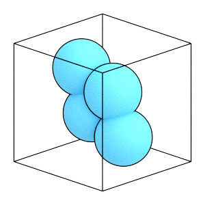
The remainder of this tutorial section demonstrates these steps for this body:
[3]:
general_positions = numpy.array([[.5, .5, 0], [-.5, -.5, 0], [-1, 1, 0],
                                 [1, -1, 0]])
particle_mass = 1
particle_radius = 1
[4]:
render_rigid_body(general_positions)
[4]:
Step 1: Compute the inertia tensor
HOOMD-blue makes no assumptions about the distribution of mass in your body. For example, you can compute the moment of inertia assuming that each consituent particle is a uniform density ball. The moment of inertia of a single ball computed about the center of the ball is:
[5]:
I_ref = numpy.array([[2 / 5 * particle_mass * particle_radius**2, 0, 0],
                     [0, 2 / 5 * particle_mass * particle_radius**2, 0],
                     [0, 0, 2 / 5 * particle_mass * particle_radius**2]])
I_ref
[5]:
array([[0.4, 0. , 0. ],
       [0. , 0.4, 0. ],
       [0. , 0. , 0.4]])
Using the parallel axis theorem, compute the moment of inertia tensor for the general body as a sum of constituent particle inertia tensors: \(I = I_{ref} + m[(D\cdot D)E_3 - D\otimes D]\)
\(I_{ref}\) is the reference moment of inertia, m is the mass, D is the displacement (i.e. the position of the constituent particle in body coordinates) and \(E_3\) is the identity matrix.
[6]:
I_general = numpy.zeros(shape=(3, 3))
for r in general_positions:
    I_general += I_ref + particle_mass * (numpy.dot(r, r) * numpy.identity(3)
                                          - numpy.outer(r, r))

I_general
[6]:
array([[4.1, 1.5, 0. ],
       [1.5, 4.1, 0. ],
       [0. , 0. , 6.6]])
Notice that some of the off-diagonal elements are non-zero. These body coordinates are not appropriate for use in HOOMD-blue.
Step 2: Diagonalize the moment of inertia
First, find the eigenvalues of the general moment of inertia:
[7]:
I_diagonal, E_vec = numpy.linalg.eig(I_general)
The diagonalized moment of inertia are the \([I_{xx}, I_{yy}, I_{zz}]\) needed by HOOMD-blue:
[8]:
I_diagonal
[8]:
array([5.6, 2.6, 6.6])
The transpose of the eigenvector matrix rotates the original particles into the frame where the inertia tensor is diagonalized:
[9]:
R = E_vec.T
Rotate the particles by this matrix:
[10]:
diagonal_positions = numpy.dot(R, general_positions.T).T
diagonal_positions
[10]:
array([[ 7.07106781e-01, -5.55111512e-17,  0.00000000e+00],
       [-7.07106781e-01,  5.55111512e-17,  0.00000000e+00],
       [ 1.11022302e-16,  1.41421356e+00,  0.00000000e+00],
       [-1.11022302e-16, -1.41421356e+00,  0.00000000e+00]])
[11]:
render_rigid_body(diagonal_positions)
[11]:
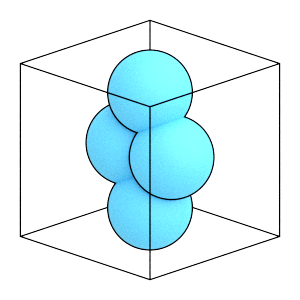
The rigid body has now been aligned its principle rotational axes with the x, y, and z body axes. Use diagonal_positionsas body coordinates along with I_diagonal as the central particle’s moment_inertia.
To check, let’s confirm that the directly calculated moment of inertia of the new coordinates is diagonal.
[12]:
I_check = numpy.zeros(shape=(3, 3))
for r in diagonal_positions:
    I_check += I_ref + particle_mass * (numpy.dot(r, r) * numpy.identity(3)
                                        - numpy.outer(r, r))

I_check
[12]:
array([[ 5.60000000e+00, -2.35513869e-16,  0.00000000e+00],
       [-2.35513869e-16,  2.60000000e+00,  0.00000000e+00],
       [ 0.00000000e+00,  0.00000000e+00,  6.60000000e+00]])
This moment of inertia is diagonal within numerical precision.
When the diagonalization process produces very small numerical values for the diagonal elements, set them to 0 explicitly to disable those degrees of freedom. Otherwise, HOOMD-blue will attempt to integrate them, resulting in numerical instabilities.
This is the end of the introduction to the modelling rigid bodies tutorial! It described the properties of rigid bodies, showed how to run a simulation of dimers, and demonstrated how to diagonalize the moment of inertia of general bodies. See the other HOOMD-blue tutorials to learn about other concepts, or browse the reference documentation for more information.