Randomizing the System
Overview
Questions
How can I generate a random initial condition?
Objectives
Show how to use HPMC to randomize the initial condition.
Demonstrate how to run a simulation.
Show how to use HPMC integrator properties to examine the acceptance ratio.
Explain that short simulations at low density effectively randomize the system.
Boilerplate code
[1]:
import math

import hoomd
The render function in the next (hidden) cell will render a snapshot using fresnel.
This is not intended as a full tutorial on fresnel - see the fresnel user documentation if you would like to learn more.
Method
The previous section of this tutorial placed all the particles on a simple cubic lattice. This is a convenient way to place non-overlapping particles, but it starts the simulation in a highly ordered state. You should randomize the the system enough so that it forgets this initial state and self-assembly can proceed without influence by the initial condition.
You cannot draw random numbers trivially for the particle positions, as that will result in overlaps between particles. Instead, start from the lattice and use HPMC to move particles randomly while ensuring that they do not overlap. In low density configurations, like the lattice generated in the previous section, a short simulation will quickly randomize the system.
Set up the simulation
The following code block creates the Simulation, configures the HPMC integrator, and initializes the system state from lattice.gsd as has been discussed in previous sections in this tutorial:
[4]:
cpu = hoomd.device.CPU()
sim = hoomd.Simulation(device=cpu, seed=20)

mc = hoomd.hpmc.integrate.ConvexPolyhedron()
mc.shape['octahedron'] = dict(vertices=[
    (-0.5, 0, 0),
    (0.5, 0, 0),
    (0, -0.5, 0),
    (0, 0.5, 0),
    (0, 0, -0.5),
    (0, 0, 0.5),
])

sim.operations.integrator = mc
sim.create_state_from_gsd(filename='lattice.gsd')
Run the simulation
Save a snapshot of the current state of the system. This tutorial uses this later to see how far particles have moved.
[5]:
initial_snapshot = sim.state.get_snapshot()
Run the simulation to randomize the particle positions and orientations. The run method takes the number of steps to run as an argument. 10,000 steps is enough to randomize a low density system:
[6]:
sim.run(10e3)
You can query properties of the HPMC integrator to see what it did. translate_moves is a tuple with the number of accepted and rejected translation moves. The acceptance ratio, the fraction of attempted moves which are accepted, is very high at this low density.
[7]:
mc.translate_moves
[7]:
(2412359, 147260)
[8]:
mc.translate_moves[0] / sum(mc.translate_moves)
[8]:
0.9424680001203304
rotate_moves similarly provides the number of accepted and rejected rotation moves.
[9]:
mc.rotate_moves
[9]:
(2489315, 71066)
[10]:
mc.rotate_moves[0] / sum(mc.rotate_moves)
[10]:
0.9722439746272137
overlaps reports the number of overlapping particle pairs in the state. There are no overlaps in the final configuration:
[11]:
mc.overlaps
[11]:
0
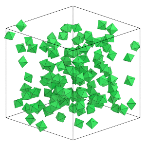
The final configuration
Look at the final particle positions and orientations and see how they have changed:
[12]:
final_snapshot = sim.state.get_snapshot()
render(final_snapshot)
[12]:
[13]:
initial_snapshot.particles.position[0:4]
[13]:
array([[-3.5999999 , -3.5999999 , -3.5999999 ],
       [-3.5999999 , -3.5999999 , -2.4000001 ],
       [-3.5999999 , -3.5999999 , -1.20000005],
       [-3.5999999 , -3.5999999 ,  0.        ]])
[14]:
final_snapshot.particles.position[0:4]
[14]:
array([[-0.34045062, -3.40372881,  0.97162443],
       [ 0.37658316,  2.24546797, -1.57884474],
       [ 2.89672535, -0.69444436, -3.18158696],
       [-1.60254438, -1.12832378, -0.05738665]])
[15]:
initial_snapshot.particles.orientation[0:4]
[15]:
array([[1., 0., 0., 0.],
       [1., 0., 0., 0.],
       [1., 0., 0., 0.],
       [1., 0., 0., 0.]])
[16]:
final_snapshot.particles.orientation[0:4]
[16]:
array([[-0.1604707 ,  0.00679003,  0.56703214,  0.80788464],
       [ 0.30537333,  0.06005637,  0.66613445, -0.6777944 ],
       [-0.83000904, -0.09179543,  0.40795323, -0.36909723],
       [ 0.52359268, -0.49392678, -0.68970674, -0.07868712]])
The particle positions and orientations have indeed changed significantly, telling us that the system is well randomized.
Save the final configuration to a GSD file for use in the next stage of the simulation:
[17]:
hoomd.write.GSD.write(state=sim.state, mode='xb', filename='random.gsd')
The next section of the tutorial takes random.gsd and compresses it down to a higher density.