Introduction to Rigid Bodies

Overview

Questions

• What is a rigid body?

• How do I set rigid body parameters?

• How do the rigid body parameters translate into the simulation box?

Objectives

• Define a rigid body as central particle and a set of constituent particles.

• Describe how body coordinates relate to global coordinates.

• Enumerate the properties of rigid bodies.

• Demonstrate setting the properties of a rigid dimer and creating an initial condition.

Boilerplate code

import itertools
import math

import gsd.hoomd
import hoomd
import matplotlib
import numpy

%matplotlib inline
matplotlib.style.use('ggplot')

The render function in the next (hidden) cell will render the system state using fresnel.

This is not intended as a full tutorial on fresnel - see the fresnel user documentation if you would like to learn more.

Introduction

A rigid body is an incompressible body composed of one central and one or more constituent particles. All particles in a given rigid body interact with all other particles in the simulation. In molecular dynamics simulations, the central particle translates and rotates in response to the net force and torque on the body. The constituent particles follow the central particle.

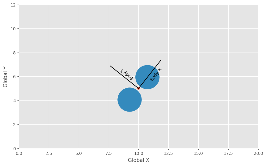
Coordinate systems

You define the positions and orientations of the constituent particles in body coordinates, a coordinate system where the (0,0,0) is at the position of the central particle and the body is in a reference orientation.

For example, define the positions of two points in a rigid dimer:

dimer_positions = [[-1.2, 0, 0], [1.2, 0, 0]]

Each instance of a rigid body in a simulation is placed in the system global coordinates, located by the position and orientation of the central particle.

central_position = [10, 5, 0]
central_rotation = 0.9

To demonstrate, the following code block computes the global positions of the the dimer at the given central position and rotation (in 2D).

cos_theta = math.cos(central_rotation)
sin_theta = math.sin(central_rotation)

global_positions = []
for i in range(len(dimer_positions)):
    x, y = dimer_positions[i][:2]

    global_positions.append(
        [[central_position[0] + (x * cos_theta - y * sin_theta)],
         [central_position[1] + (y * cos_theta + x * sin_theta)]])

Visualize the configuration:

fig = matplotlib.figure.Figure(figsize=(10, 6.18), dpi=100)
ax = fig.add_subplot(aspect='equal')

ax.plot([central_position[0], central_position[0] - 3 * sin_theta],
        [central_position[1], central_position[1] + 3 * cos_theta],
        color='k')

ax.plot([central_position[0], central_position[0] + 3 * cos_theta],
        [central_position[1], central_position[1] + 3 * sin_theta],
        color='k')

ax.text(central_position[0] + 1.5 * cos_theta,
        central_position[1] + 1.5 * sin_theta,
        'Body X',
        rotation=central_rotation * 180 / math.pi,
        verticalalignment='center')

ax.text(central_position[0] - 2 * sin_theta,
        central_position[1] + 2 * cos_theta,
        'Body Y',
        rotation=central_rotation * 180 / math.pi + 90,
        verticalalignment='center')

ax.add_patch(
    matplotlib.patches.Circle((central_position[0], central_position[1]),
                              0.1,
                              color='C0'))

for position in global_positions:
    ax.add_patch(
        matplotlib.patches.Circle((position[0], position[1]), 1.0, color='C1'))

ax.set_xlim(0, 20)
ax.set_ylim(0, 12)

ax.set_xlabel('Global X')
ax.set_ylabel('Global Y')

fig

Properties of rigid bodies

The following rigid body properties are given by the properties of the central particle:

• Mass - the total mass of the rigid body.

• Moment of inertia tensor - how mass is distributed throughout the rigid body.

• Velocity - velocity of the center of mass of the rigid body.

• Angular momentum - angular momentum of the rigid body.

• Position - the position in global coordinates. Example: position = [1, 2, -3]

• Orientation - a quaternion that rotates the rigid body about the central particle. Example: orientation = [1, 0, 0, 0]

The following constituent particle properties are given by the properties of a given rigid body type:

• Constituent Particle Positions - The vector from the center of the rigid body to the constituent particle in body coordinates.

• Constituent Particle Orientation - A quaternion that rotates the constituent particle about its center.

Defining properties of the rigid dimer

Let each constituent particle in the dimer be a point particle of type A with mass 1 at the constituent positions previously defined in dimer_positions. Each dimer will be located at the position of a particle of type dimer.

Let’s create an initial configuration of dimers. Start with a snapshot containing both particle types:

snapshot = gsd.hoomd.Snapshot()
snapshot.particles.types = ['dimer', 'A']

Place dimer particles (typeid=0) in the simulation box. Place them far enough apart so that the A particles will not touch in the initial condition:

m = 4
N_particles = m**3
spacing = 5
K = math.ceil(N_particles**(1 / 3))
L = K * spacing
x = numpy.linspace(-L / 2, L / 2, K, endpoint=False)
position = list(itertools.product(x, repeat=3))
position = numpy.array(position) + [spacing / 2, spacing / 2, spacing / 2]
snapshot.particles.N = N_particles
snapshot.particles.position = position[0:N_particles, :]
snapshot.particles.typeid = [0] * N_particles
snapshot.configuration.box = [L, L, L, 0, 0, 0]

With two mass 1 particles, the total mass of the body is 2. Set the mass of each instance of the body:

snapshot.particles.mass = [2] * N_particles

The moment of inertia of a point particle about a given axis is given by \(I_i = m r_i^2\), where \(r_i\) is the distance of the point from the axis. More generally, the moment of inertia is a tensor and includes off-diagonal values (you will learn more about this in a later tutorial section).

Compute the moment of inertia of the dimer:

mass = 1
I = numpy.zeros(shape=(3, 3))
for r in dimer_positions:
    I += mass * (numpy.dot(r, r) * numpy.identity(3) - numpy.outer(r, r))
I

array([[0.  , 0.  , 0.  ],
       [0.  , 2.88, 0.  ],
       [0.  , 0.  , 2.88]])

In this case, the tensor is diagonal. This is important as HOOMD-blue assumes that bodies have a diagonal moment of inertia in body coordinates in the form: \([I_{xx}, I_{yy}, I_{zz}]\). Set the moments of inertia of each body in the snapshot:

snapshot.particles.moment_inertia = [I[0, 0], I[1, 1], I[2, 2]] * N_particles

Notice that \(I_{xx}\) is zero for this dimer while \(I_{yy}\) and \(I_{zz}\) are non-zero. HOOMD-blue checks which moments of inertia are non-zero and integrates degrees of freedom only for those axes with non-zero moments of inertia. In this example, the dimer will rotate about the body’s y and z axes, but not x.

HOOMD-blue represents orientations with quaternions. The quaternion \([1, 0, 0, 0]\) is the identity. Set the orientation of each body in the snapshot to the identity:

snapshot.particles.orientation = [(1, 0, 0, 0)] * N_particles

Write the rigid centers to a GSD file for later use:

with gsd.hoomd.open(name='dimer_centers.gsd', mode='xb') as f:
    f.append(snapshot)

The hoomd.md.constrain.Rigid class is responsible for applying the rigid body constraints:

rigid = hoomd.md.constrain.Rigid()

Set the constituent particle properties in body coordinates for the rigid body type:

rigid.body['dimer'] = {
    "constituent_types": ['A', 'A'],
    "positions": dimer_positions,
    "orientations": [(1.0, 0.0, 0.0, 0.0), (1.0, 0.0, 0.0, 0.0)],
    "charges": [0.0, 0.0],
    "diameters": [1.0, 1.0]
}

Rigid will use positions and orientations to set the global positions and orientations of all constituent particles on every time step. The constituent_types, charges, and diameters fields provide a template for create_bodies (see below).

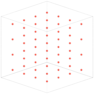
Placing constituent particles in the initial condition

So far, our snapshot has only the dimer central particles:

sim = hoomd.Simulation(device=hoomd.device.CPU(), seed=4)
sim.create_state_from_gsd(filename='dimer_centers.gsd')
render(sim.state.get_snapshot())

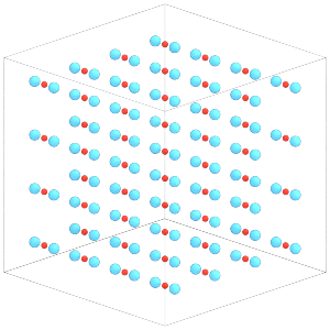
Rigid.create_bodies will place constituent particles in the simulation state:

rigid.create_bodies(sim.state)

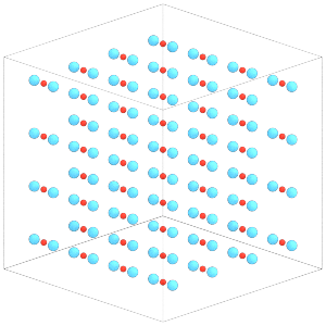
Each central particle now has the two constituent particles of the dimer placed around it:

render(sim.state.get_snapshot())

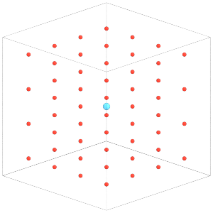
Understand that Rigid will overwrite the positions and orientations of the constituent particles in the simulation state. To demonstrate, let’s modify the positions of the constituents:

with sim.state.cpu_local_snapshot as snapshot:
    typeid = snapshot.particles.typeid
    snapshot.particles.position[typeid == 1] = [0, 0, 0]

render(sim.state.get_snapshot())

Set the rigid constraint with the MD integrator so it will take effect on the simulation. The next section of this tutorial will explain these steps in more detail:

integrator = hoomd.md.Integrator(dt=0.005, integrate_rotational_dof=True)
integrator.rigid = rigid
sim.operations.integrator = integrator

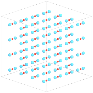
Rigid will apply the rigid body constraints at the start of a simulation run and on every timestep. Calling sim.run(0) will restore the constituent particle positions:

sim.run(0)
render(sim.state.get_snapshot())

To change the position or orientation of a given body, change the properties of the central particle:

with sim.state.cpu_local_snapshot as snapshot:
    typeid = snapshot.particles.typeid
    snapshot.particles.orientation[typeid == 0] = [
        0.70710678, 0., 0.70710678, 0.
    ]

Again, execute sim.run(0) for the changes to take effect on the constituent particles.

sim.run(0)
render(sim.state.get_snapshot())

Write the configuration to a file for use in the next tutorial section:

hoomd.write.GSD.write(state=sim.state, mode='xb', filename='lattice.gsd')

In this section, you learned how HOOMD-blue composes rigid bodies of central and constituent particles and about all the properties of those bodies. You also saw how to define these parameters and how Rigid updates them in the simulation state. The next section will explain how to run a molecular dynamics simulation of this system.