Logging to a GSD file
Overview
Questions
What is a Logger?
How can I write thermodynamic and other quantities to a file?
How can I access that data?
Objectives
Describe and give examples of loggable quantities.
Show how to add quantities to a Logger.
Demonstrate GSD as a log writer.
Explain how to read logged quantities from GSD files.
Describe how namespaces appear in the names of the logged quantities.
Boilerplate code
[1]:
import gsd.hoomd
import hoomd
import matplotlib

%matplotlib inline
matplotlib.style.use('ggplot')
Introduction
HOOMD separates logging into three parts: Loggable quantities, the Logger class, and Writers.
Loggable quantities are values computed during a simulation.
The Logger class provides a way to collect and name quantities of interest.
Writers write these values out in a format you can use.
In this section, you will use the GSD Writer to capture the values of quantities during a simulation run for later analysis.
Define the Simulation
This tutorial executes the Lennard-Jones particle simulation from a previous tutorial. See Introducing Molecular Dyamics for a complete description of this code.
[3]:
cpu = hoomd.device.CPU()
sim = hoomd.Simulation(device=cpu)
sim.create_state_from_gsd(
    filename='../01-Introducing-Molecular-Dynamics/random.gsd')

integrator = hoomd.md.Integrator(dt=0.005)
cell = hoomd.md.nlist.Cell(buffer=0.4)
lj = hoomd.md.pair.LJ(nlist=cell)
lj.params[('A', 'A')] = dict(epsilon=1, sigma=1)
lj.r_cut[('A', 'A')] = 2.5
integrator.forces.append(lj)
nvt = hoomd.md.methods.NVT(kT=1.5, filter=hoomd.filter.All(), tau=1.0)
integrator.methods.append(nvt)
sim.operations.integrator = integrator
sim.run(0)
Loggable quantities
Many classes in HOOMD-blue provide special properties called loggable quantities. For example, the Simulation class provides timestep, tps, and others. The reference documentation labels each of these as Loggable. You can also examine the loggables property to determine the loggable quantities:
[4]:
sim.loggables
[4]:
{'timestep': 'scalar',
 'seed': 'scalar',
 'tps': 'scalar',
 'walltime': 'scalar',
 'final_timestep': 'scalar'}
The ThermodynamicQuantities class computes a variety of thermodynamic properties in MD simulations. These are all loggable.
[5]:
thermodynamic_properties = hoomd.md.compute.ThermodynamicQuantities(
    filter=hoomd.filter.All())
sim.operations.computes.append(thermodynamic_properties)
thermodynamic_properties.loggables
[5]:
{'kinetic_temperature': 'scalar',
 'pressure': 'scalar',
 'pressure_tensor': 'sequence',
 'kinetic_energy': 'scalar',
 'translational_kinetic_energy': 'scalar',
 'rotational_kinetic_energy': 'scalar',
 'potential_energy': 'scalar',
 'degrees_of_freedom': 'scalar',
 'translational_degrees_of_freedom': 'scalar',
 'rotational_degrees_of_freedom': 'scalar',
 'num_particles': 'scalar',
 'volume': 'scalar'}
Loggable quantities are class properties or methods. You can directly access them in your code.
[6]:
sim.timestep
[6]:
10000
[7]:
thermodynamic_properties.kinetic_temperature
[7]:
1.4796558111045974
Each loggable quantity has a category, which is listed both in the reference documentation and in loggables. The category is a string that identifies the quantity’s type or category. Example categories include: * scalar - numbers * sequence - arrays of numbers * string - strings of characters * particle - arrays of per-particle values
Add quantities to a Logger
Add each of the quantities you would like to store to a Logger. The Logger will maintain these quantities in a list and provide them to the Writer when needed.
[8]:
logger = hoomd.logging.Logger()
You can add loggable quantities from any number of objects to a Logger. Logger uses the namespace of the class to assign a unique name for each quantity. Call add to add all quantities provided by thermodynamic_properties:
[9]:
logger.add(thermodynamic_properties)
You can also select specific quantities to add with the quantities argument. Add only the timestep and walltime quantities from Simulation:
[10]:
logger.add(sim, quantities=['timestep', 'walltime'])
Writing log quantities to a GSD file
GSD files always store trajectories of particle properties. Set the log attribute and GSD will also store the selected quantities.
You can store only the logged quantities by using the Null filter to select no particles for the trajectory. This way, you can log thermodynamic properties at a high rate and keep the file size small.
[11]:
gsd_writer = hoomd.write.GSD(filename='log.gsd',
                             trigger=hoomd.trigger.Periodic(1000),
                             mode='xb',
                             filter=hoomd.filter.Null())
sim.operations.writers.append(gsd_writer)
Assign the logger to include the logged quanties in the GSD file:
[12]:
gsd_writer.log = logger
The writer triggers and writes to the log file when the simulation runs:
[13]:
sim.run(100000)
Reading logged data from a GSD file
You need to close the GSD file that gsd_writer has open before you can read it. The following code block deletes the simulation and operations manually so that it is safe to open the file for reading later in this notebook.
In typical workflows, you will run separate simulation and analysis scripts and the GSD file will be closed when your simulation script exits.
[14]:
del sim, gsd_writer, thermodynamic_properties, logger
del integrator, nvt, lj, cell, cpu
Use the gsd package to open the file:
[15]:
traj = gsd.hoomd.open('log.gsd', 'rb')
Each frame in the trajectory has a log dictionary that maps quantity names to values. Inspect this dictionary in the first frame:
[16]:
traj[0].log
[16]:
{'md/compute/ThermodynamicQuantities/kinetic_temperature': array([1.48311699]),
 'md/compute/ThermodynamicQuantities/pressure': array([0.51801307]),
 'md/compute/ThermodynamicQuantities/pressure_tensor': array([ 0.57363457,  0.0193231 , -0.00974054,  0.44857891,  0.14908453,
         0.53182573]),
 'md/compute/ThermodynamicQuantities/kinetic_energy': array([567.29224759]),
 'md/compute/ThermodynamicQuantities/translational_kinetic_energy': array([567.29224759]),
 'md/compute/ThermodynamicQuantities/rotational_kinetic_energy': array([0.]),
 'md/compute/ThermodynamicQuantities/potential_energy': array([-528.13490623]),
 'md/compute/ThermodynamicQuantities/degrees_of_freedom': array([765.]),
 'md/compute/ThermodynamicQuantities/translational_degrees_of_freedom': array([765.]),
 'md/compute/ThermodynamicQuantities/rotational_degrees_of_freedom': array([0.]),
 'md/compute/ThermodynamicQuantities/num_particles': array([256]),
 'md/compute/ThermodynamicQuantities/volume': array([753.57109477]),
 'Simulation/timestep': array([11000]),
 'Simulation/walltime': array([0.227067])}
The dictionary keys are verbose names that include the namespace of the class which computed the quantity, where . has been replaced with /. For example, access the potential energy computed by ThermodynamicQuantities with the key md/compute/ThermodynamicQuantities/potential_energy.
[17]:
traj[0].log['md/compute/ThermodynamicQuantities/potential_energy']
[17]:
array([-528.13490623])
GSD stores all quantities in arrays. It stores scalar quantities such as the system potential energy in length 1 arrays (above) while it stores vector and other array quantities as appropriately sized arrays:
[18]:
traj[0].log['md/compute/ThermodynamicQuantities/pressure_tensor']
[18]:
array([ 0.57363457,  0.0193231 , -0.00974054,  0.44857891,  0.14908453,
        0.53182573])
GSD provides logged quantities individually at each frame in the file. You can convert this to time-series data with a loop and then plot or analyze it:
[19]:
timestep = []
walltime = []
potential_energy = []

for frame in traj:
    timestep.append(frame.configuration.step)
    walltime.append(frame.log['Simulation/walltime'][0])
    potential_energy.append(
        frame.log['md/compute/ThermodynamicQuantities/potential_energy'][0])
[20]:
fig = matplotlib.figure.Figure(figsize=(10, 6.18))
ax = fig.add_subplot()
ax.plot(timestep, potential_energy)
ax.set_xlabel('timestep')
ax.set_ylabel('potential energy')
fig
[20]:
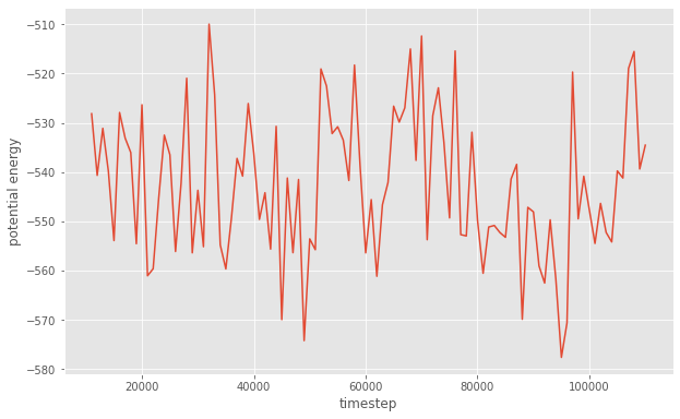
In this section, you have logged quantities to a GSD file during a simulation run and analyzed that data as a time series. The next section of this tutorial shows you how to save per-particle quantities associated with specific system configurations.