Compressing the System
Overview
Questions
How do I compress the system to a target density?
Objectives
Describe how Variants describe values that vary with the timestep.
Show how to use BoxResize with a Ramp variant to slowly compress the system to the target volume.
Demonstrate the crystallization of Lennard-Jones particles
Boilerplate code
[1]:
import math

import fresnel
import hoomd
import matplotlib

%matplotlib inline
matplotlib.style.use('ggplot')
The render function in the next (hidden) cell will render the system state using fresnel.
This is not intended as a full tutorial on fresnel - see the fresnel user documentation if you would like to learn more.
Procedure
random.gsd, generated by the previous section of this tutorial has particles randomly placed in a low density fluid state. To find the crystalline state, you need to compress the system to a higher density. If you were to immediately scale the system to the target density, the particle’s hard cores would overlap and the integrator would be become unstable. A more effective strategy gradually resizes the simulation box a little at a time over the course of a simulation, allowing any slight
overlaps to relax.
Initialize the simulation
Configure this simulation to run on the CPU.
[3]:
cpu = hoomd.device.CPU()
sim = hoomd.Simulation(device=cpu)
sim.create_state_from_gsd(filename='random.gsd')
Set up the molecular dynamics simulation, as discussed in the previous sections of this tutorial:
[4]:
integrator = hoomd.md.Integrator(dt=0.005)
cell = hoomd.md.nlist.Cell(buffer=0.4)
lj = hoomd.md.pair.LJ(nlist=cell)
lj.params[('A', 'A')] = dict(epsilon=1, sigma=1)
lj.r_cut[('A', 'A')] = 2.5
integrator.forces.append(lj)
nvt = hoomd.md.methods.NVT(kT=1.5, filter=hoomd.filter.All(), tau=1.0)
integrator.methods.append(nvt)
sim.operations.integrator = integrator
Variants
The BoxResize class performs scales the simulation box. You provide a Variant that tells BoxResize how to interpolate between two boxes, box1 and box2, over time. A Variant is a scalar-valued function of the simulation timestep. BoxResize sets box1 when the function is at its minimum, box2 when the function is at its maximum, and linearly interpolates between the two boxes for intermediate values.
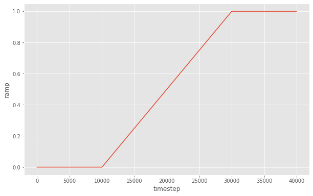
Use the Ramp variant to define a function that ramps from one value to another over a given number of steps. Note that this simulation does not start at timestep 0, random.gsd was saved after running a number of steps to randomize the system in the previous section:
[5]:
sim.timestep
[5]:
10000
Create a Ramp that starts at this step and ends 100,000 steps later:
[6]:
ramp = hoomd.variant.Ramp(A=0, B=1, t_start=sim.timestep, t_ramp=20000)
Here is what the ramp looks like as a function of timestep:
[7]:
steps = range(0, 40000, 20)
y = [ramp(step) for step in steps]

fig = matplotlib.figure.Figure(figsize=(10, 6.18))
ax = fig.add_subplot()
ax.plot(steps, y)
ax.set_xlabel('timestep')
ax.set_ylabel('ramp')
fig
[7]:
Gradually resize the simulation box
Now, you need to determine the initial simulation box box1 and final simulation box at the target density box2. This is the initial number density \(\rho\) of the current simulation box:
[8]:
rho = sim.state.N_particles / sim.state.box.volume
rho
[8]:
0.3397157902913389
Create a new Box at the target number density:
[9]:
initial_box = sim.state.box
final_box = hoomd.Box.from_box(initial_box)  # make a copy of initial_box
final_rho = 1.2
final_box.volume = sim.state.N_particles / final_rho
To avoid destabilizing the integrator with large forces due to large box size changes, scale the box with a small period.
[10]:
box_resize_trigger = hoomd.trigger.Periodic(10)
Construct the BoxResize updater and add it to the simulation.
[11]:
box_resize = hoomd.update.BoxResize(box1=initial_box,
                                    box2=final_box,
                                    variant=ramp,
                                    trigger=box_resize_trigger)
sim.operations.updaters.append(box_resize)
Run the simulation to compress the box.
[12]:
sim.run(10001)
At the half way point of the ramp, the variant is 0.5 and the current box lengths are half way between the initial and final ones:
[13]:
ramp(sim.timestep - 1)
[13]:
0.5
[14]:
current_box = sim.state.box
(current_box.Lx - initial_box.Lx) / (final_box.Lx - initial_box.Lx)
[14]:
0.5
Finish the rest of the compression:
[15]:
sim.run(10000)
The current box matches the final box:
[16]:
sim.state.box == final_box
[16]:
True
The system is at a higher density:
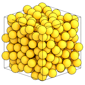
[17]:
render(sim.state.get_snapshot())
[17]:
Now that the system has reached the target volume, remove the BoxResize updater from the simulation:
[18]:
sim.operations.updaters.remove(box_resize)
Equilibrating the system
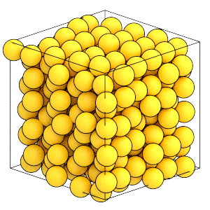
Run the simulation for a longer time and see if it self assembles the ordered fcc structure:
This cell may require several minutes to complete.
[19]:
sim.run(5e5)
Here is what the final state of the system looks like:
[20]:
render(sim.state.get_snapshot())
[20]:
Analyzing the simulation results
Is this the fcc structure? Did the system reach equilibrium? These are topics covered in the Introducing HOOMD-blue tutorial. Consider it an exercise to modify this example and implement that analysis here. You will need to save a GSD file with the simulation trajectory, then use freud’s SolidLiquid order parameter to identify when the ordered structure appears.
This is the end of the introducing molecular dynamics tutorial! It described molecular dynamics simulations, demonstrated how to initialize, randomize, compress, and equilibrate a system of Lennard-Jones particles. See the other HOOMD-blue tutorials to learn about other concepts, or browse the reference documentation for more information.