Analyzing Trajectories
Overview
Questions
How can I analyze trajectories?
Objectives
Describe how to access trajectory frames in GSD.
Examine the trajectory with freud and fresnel.
Boilerplate code
[1]:
import math

import fresnel
import freud
import gsd.hoomd
import matplotlib

%matplotlib inline
matplotlib.style.use('ggplot')
The render function in the next (hidden) cell will render a snapshot using fresnel. render_movie will render a sequence of frames as an animated GIF. These methods accept a particles argument that filters out which particles to display.
This is not intended as a full tutorial on fresnel - see the fresnel user documentation if you would like to learn more.
Equilibration challenges
In the previous section, you ran the hard octahedra system for many time steps to equilibrate it and saved the trajectory in trajectory.gsd. Is the final state you obtained actually an equilibrium state? Statistical mechanics tells us that as long as our system is ergodic it will eventually achieve equilibrium. You need to analyze this trajectory to determine if you have achieved the ordered equilibrium structure.
Tools
There are many tools that can read GSD files and analyze or visualize the simulations, and many more Python packages that can work with the numerical data. This tutorial will show you how to use freud to determine which particles are in a solid-like environment and fresnel to render system configurations. The freud Python package provides a simple, flexible, powerful set of tools for analyzing trajectories obtained from molecular dynamics or Monte Carlo simulations. The fresnel Python package produces publication quality renders with soft lighting, depth of field and other effects.
While outside the scope of this tutorial, you might want to use tools such as OVITO or VMD to visualize the trajectory interactively. OVITO has built-in support for GSD files. The gsd-vmd plugin adds support to VMD.
Read the trajectory
Use GSD to open the trajectory generated by the previous section of this tutorial.
[3]:
traj = gsd.hoomd.open('trajectory.gsd')
You can index into the frames of the trajectory like a list. See how many frames exist in the trajectory:
[4]:
len(traj)
[4]:
105
Ergodicity
A system is ergodic when it can explore all possible states by making small moves from one to another. In HPMC simulations, low volume fraction simulations are ergodic while very high volume fraction ones are not. At high volume fractions, there isn’t enough free space for the particles to rearrange so they get stuck in local configurations.
Visualize the motion of just a few particles to see if they appear stuck or if they are freely moving about the box:
[5]:
render_movie(traj[0:50:5], particles=[12, 18])
Good! Over the first part of the simulation (while the system is still fluid), individual particles are able to move a significant distance and explore many different orientations. This indicates that our system is ergodic.
Simulation length
How can you tell if you have run long enough to equilibrate the system? The hard octahedra system forms the bcc structure by nucleation and growth. Nucleation is a rare event, so you need to keep running the simulation until it occurs. If you ran this simulation many times with different random seeds, each would take a different number of steps to nucleate. You need to examine the simulation trajectory in detail to determine if you have run it long enough.
[6]:
render_movie(traj[0:100:12])
Can you see the system ordering? The orientations of the octahedra appear to quickly snap to face the same direction and the particle positions line up on evenly spaced planes. You can use freud’s SolidLiquid analysis method to quantitatively identify which particles are in the solid structure.
Loop over all of the frames in the file and create a boolean array that indicates which particles are in a solid environment:
[7]:
solid = freud.order.SolidLiquid(l=6, q_threshold=0.7, solid_threshold=6)
is_solid = []
for frame in traj:
    solid.compute(system=(frame.configuration.box, frame.particles.position),
                  neighbors=dict(mode='nearest', num_neighbors=8))
    is_solid.append(solid.num_connections > solid.solid_threshold)
Plot the total number of particles in a solid environment over time:
[8]:
fig = matplotlib.figure.Figure(figsize=(10, 6.18))
ax = fig.add_subplot()
num_solid = numpy.array([numpy.sum(a) for a in is_solid])
ax.plot(num_solid)
ax.set_xlabel('frame')
ax.set_ylabel('number of particles in a solid environment')
fig
[8]:
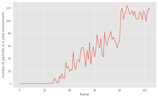
This plot confirms what you saw visually and what you should expect in a system that nucleates and grows a crystal. There is no solid at the beginning of the simulation. Then a solid cluster forms and grows quickly to fill the box.
Visualize just the solid particles to see this more clearly:
[9]:
start_frame = int(numpy.argmax(num_solid > 4))
end_frame = int(numpy.argmax(num_solid == numpy.max(num_solid)))
step = int((end_frame - start_frame) / 6)
render_movie(traj[start_frame:end_frame:step],
             is_solid=is_solid[start_frame:end_frame:step])
This is the end of the first tutorial! It covered the core HOOMD-blue objects, described hard particle Monte Carlo simulations, and demonstrated how to initialize, randomize, compress, equilibrate, and analyze a system of self-assembling hard octahedra. See the other HOOMD-blue tutorials to learn about other concepts, or browse the reference documentation for more information.