Molecular Dynamics Simulations
Overview
Questions
What is molecular dynamics?
How do I set up a molecular dynamics simulation in HOOMD-blue?
Objectives
Describe the equations of motion of the system and HOOMD-blue solves them with time steps.
Define forces, potential energy and explain how HOOMD-blue evaluates pair potentials within a cutoff.
Explain how the MD Integrator and integration methods solve the equations of motion and allow for different thermodynamic ensembles.
Boilerplate code
[1]:
import hoomd
import matplotlib
import numpy

%matplotlib inline
matplotlib.style.use('ggplot')
Equations of motion
Molecular dynamics simulations model the movement of particles over time by solving the equations of motion numerically, advancing the state of the system forward by time dt on each time step. You can use molecular dynamics to model dynamic, time dependent processes (like fluid flow) or thermodynamic equilibrium states (like crystals). This tutorial models a system of Lennard-Jones particles crystallizing.
The Integrator class in the md package implements molecular dynamics integration in HOOMD-blue:
[2]:
integrator = hoomd.md.Integrator(dt=0.005)
The dt property sets the step size \(\Delta t\):
[3]:
integrator.dt
[3]:
0.005
Forces
The force term in the equations of motion determines how particles interact. The forces Integrator property is the list of forces applied to the system. The default is no forces:
[4]:
integrator.forces[:]
[4]:
[]
You can add any number of Force objects to this list. Each will compute forces on all particles in the system state. Integrator will add all of the forces together into the net force used in the equations of motion.
HOOMD-blue provides a number of forces that are derived from potential energy. Pair potentials define the functional form of the potential energy between a single pair of particles given their separation distance r. The Lennard-Jones potential is:
[5]:
sigma = 1
epsilon = 1
r = numpy.linspace(0.95, 3, 500)
V_lj = 4 * epsilon * ((sigma / r)**12 - (sigma / r)**6)

fig = matplotlib.figure.Figure(figsize=(10, 6.18))
ax = fig.add_subplot()
ax.plot(r, V_lj)
ax.set_xlabel('r')
ax.set_ylabel('V')
fig
[5]:
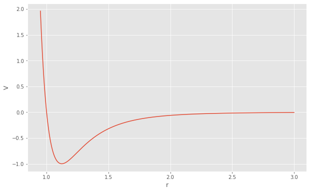
While pair potentials are nominally defined between all pairs of particles, Molecular dynamics simulations evaluate short ranged pair potentials only for \(r \lt r_{\mathrm{cut}}\) to make the computation fast through the use of a neighbor list. By default, HOOMD-blue introduces a discontinuity in V at \(r=r_{\mathrm{cut}}\), though there are options to shift or smooth the potential at the cutoff.
HOOMD-blue provides several neighbor list options to choose from. Cell performs well in most situations. The buffer parameter sets an extra distance to include in the neighbor list, so it can be used for multiple timesteps without recomputing neighbors. Choose a value that minimizes the time to execute your simulation.
[6]:
cell = hoomd.md.nlist.Cell(buffer=0.4)
Construct the LJ pair force object to compute the Lennard-Jones interactions:
[7]:
lj = hoomd.md.pair.LJ(nlist=cell)
Pair potentials accept parameters for every pair of particle types in the simulation. Define a single A-A interaction for this tutorial:
[8]:
lj.params[('A', 'A')] = dict(epsilon=1, sigma=1)
lj.r_cut[('A', 'A')] = 2.5
Add the force to the Integrator:
[9]:
integrator.forces.append(lj)
Now, the Integrator will compute the net force term using the Lennard-Jones pair force.
Integration methods
HOOMD-blue provides a number of integration methods, which define the equations of motion that apply to a subset of the particles in the system. These methods are named after the thermodynamic ensemble they implement. For example, NVE implements Newton’s laws while NVT adds a thermostat degree of freedom so the system will sample the canonical ensemble.
Lennard-Jones particles crystallize readily at constant temperature and volume. One of the points in the solid area of the phase diagram is \(kT=1.5\) at a number density \(\rho=1.2\) Apply the NVT method all particles to set the constant temperature (later sections in this tutorial will set the density):
[10]:
nvt = hoomd.md.methods.NVT(kT=1.5, filter=hoomd.filter.All(), tau=1.0)
kT is the temperature multiplied by Boltzmann’s constant and has units of energy. tau is a time constant that controls the amount of coupling between the thermostat and particle’s degrees of freedom. filter is a particle filter object that selects which particles this integration method applies to. You can apply multiple integration methods to different sets of particles or leave some particles fixed.
Add the method to the Integrator:
[11]:
integrator.methods.append(nvt)
Now, you have defined a molecular dynamics integrator with a step size dt that will use the NVT integration method on all particles interacting via the Lennard-Jones potential.
The remaining sections in this tutorial will show you how to initialize a random low density state, compress the system to a target density, and run the simulation long enough to self-assemble an ordered state.