Saving Array Quantities
Overview
Questions
How can I save per-particle quantities for later analysis?
How can I access that data?
Objectives
Show how to log per-particle properties to a GSD file.
Explain how to read logged quantities from a GSD file.
Mention that OVITO reads these quantities.
Boilerplate code
[1]:
import gsd.hoomd
import hoomd
import matplotlib
import numpy

%matplotlib inline
matplotlib.style.use('ggplot')
The render function in the next (hidden) cell will render the system state using fresnel.
This is not intended as a full tutorial on fresnel - see the fresnel user documentation if you would like to learn more.
Array quantities
You logged a 6-element array quantity in the previous section, the pressure tensor. You can also log larger arrays and per-particle quantities (e.g. energy and force) in a GSD file along with the trajectory. Then you can use utilize the data in your analysis and visualization workflow, such as using OVITO to color particles by energy or display force vectors. When using OVITO, open the GSD file and all logged quantities will be available in the inspector and for use in the pipeline.
Define the Simulation
This tutorial executes the Lennard-Jones particle simulation from a previous tutorial. See Introducing Molecular Dyamics for a complete description of this code.
[4]:
cpu = hoomd.device.CPU()
sim = hoomd.Simulation(device=cpu)
sim.create_state_from_gsd(
    filename='../01-Introducing-Molecular-Dynamics/random.gsd')

integrator = hoomd.md.Integrator(dt=0.005)
cell = hoomd.md.nlist.Cell(buffer=0.4)
lj = hoomd.md.pair.LJ(nlist=cell)
lj.params[('A', 'A')] = dict(epsilon=1, sigma=1)
lj.r_cut[('A', 'A')] = 2.5
integrator.forces.append(lj)
nvt = hoomd.md.methods.NVT(kT=1.5, filter=hoomd.filter.All(), tau=1.0)
integrator.methods.append(nvt)
sim.operations.integrator = integrator
sim.run(0)
Logging per-particle quantities
MD forces provide a number of loggable quantities including their contribution to the system energy, but also per-particle energy contributions (in energies) and per-particle forces, torques, and virials.
[5]:
lj.loggables
[5]:
{'energy': 'scalar',
 'energies': 'particle',
 'additional_energy': 'scalar',
 'forces': 'particle',
 'torques': 'particle',
 'virials': 'particle',
 'additional_virial': 'sequence'}
Add the per-particle LJ energies and forces to a logger:
[6]:
logger = hoomd.logging.Logger()
logger.add(lj, quantities=['energies', 'forces'])
Writing per-particle quantities to a GSD file
In the previous section, you used the Null filter to produce GSD file with only logged data. In this section, include all particles so that you can associate logged per-particle quantities with the particle properties.
[7]:
gsd_writer = hoomd.write.GSD(filename='trajectory.gsd',
                             trigger=hoomd.trigger.Periodic(10000),
                             mode='xb',
                             filter=hoomd.filter.All(),
                             log=logger)
sim.operations.writers.append(gsd_writer)
Run the simulation:
[8]:
sim.run(100000)
As discussed in the previous section, delete the simulation so it is safe to open the GSD file for reading in the same process.
[9]:
del sim, gsd_writer, logger, integrator, nvt, lj, cell, cpu
Reading logged data from a GSD file
Use the gsd package to open the file:
[10]:
traj = gsd.hoomd.open('trajectory.gsd', 'rb')
GSD prepends particles/ to the logged name of per-particle quantities:
[11]:
traj[0].log.keys()
[11]:
dict_keys(['particles/md/pair/LJ/energies', 'particles/md/pair/LJ/forces'])
The quantities are numpy arrays with N_particles elements. Here are a few slices:
[12]:
traj[-1].log['particles/md/pair/LJ/energies'][0:10]
[12]:
array([-3.39840884, -2.03033218, -3.15903353, -2.30211083, -0.97440217,
       -2.66465184, -1.63920762, -0.29580836, -1.14112247, -1.36468275])
[13]:
traj[-1].log['particles/md/pair/LJ/forces'][0:10]
[13]:
array([[ 1.44681031,  2.01198357,  1.0663342 ],
       [ 0.63208369,  0.6460156 ,  2.66476508],
       [-6.49972295,  1.1223018 , -2.62407767],
       [-9.1854849 , 16.68038846, -2.25596829],
       [-0.22897598, -2.50517732,  0.39782844],
       [-4.04538785, -5.33049461, -3.18924051],
       [ 0.58601689,  1.03414847, -1.51408613],
       [ 0.5440693 ,  0.40387901, -0.44558506],
       [ 4.02543414, -5.13080125,  0.17843608],
       [ 0.60842181,  0.4165125 ,  0.20256789]])
You can use these arrays as inputs to any computation or plotting tools:
[14]:
numpy.mean(traj[-1].log['particles/md/pair/LJ/forces'], axis=0)
[14]:
array([ 2.22044605e-16, 3.31223764e-16, -4.51028104e-17])
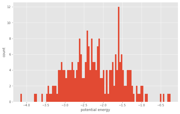
[15]:
fig = matplotlib.figure.Figure(figsize=(10, 6.18))
ax = fig.add_subplot()
ax.hist(traj[-1].log['particles/md/pair/LJ/energies'], 100)
ax.set_xlabel('potential energy')
ax.set_ylabel('count')
fig
[15]:
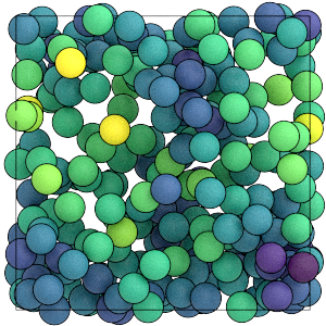
As with scalar quantities, the array quantities are stored separately in each frame. Use a loop to access a range of frames and compute time-series data or averages.
This is what the system looks like when you color the particles by the values in particles/md/pair/LJ/energies:
[16]:
render(traj[-1])
[16]:
In this section, you have logged per-particle quantities to a GSD file during a simulation run and accessed that data with a script. The next section of this tutorial demonstrates how to log particle shape information that OVITO can use.