Wall potential (MD)

Overview

Questions

• How do I apply interactions between wall geometries and particles in molecular dynamics simulations?

Objectives

• Demonstrate the use of a wall potential class.

Boilerplate code

The render function in the next (hidden) cell will render the system state using fresnel. Find the source in the hoomd-examples repository.

Place mobile particles in the center of a large simulation box:

import itertools

import gsd.hoomd
import hoomd
import numpy

L = 20
m = 10
N = m**2
x = numpy.linspace(start=-m / 2, stop=m / 2, endpoint=False, num=m) + 1 / 2
position_2d = numpy.array(list(itertools.product(x, repeat=2)))

frame = gsd.hoomd.Frame()
frame.particles.N = N
frame.particles.position = numpy.stack(
    (position_2d[:, 0], position_2d[:, 1], numpy.zeros(N)), axis=-1
)
frame.particles.types = ['mobile']
frame.configuration.box = [L, L, 0, 0, 0, 0]

with gsd.hoomd.open(name='initial_state.gsd', mode='x') as f:
    f.append(frame)

Prepare a molecular dynamics simulation:

simulation = hoomd.Simulation(device=hoomd.device.CPU(), seed=1)
simulation.create_state_from_gsd(filename='initial_state.gsd')
langevin = hoomd.md.methods.Langevin(kT=1.0, filter=hoomd.filter.All())
simulation.operations.integrator = hoomd.md.Integrator(dt=0.001, methods=[langevin])

Adding forces between particles and wall geometries

In a molecular dynamics simulation, particles move in response to applied forces. Typically, this includes a pair forces between pairs of particles:

pair_lj = hoomd.md.pair.LJ(nlist=hoomd.md.nlist.Cell(buffer=0.4), default_r_cut=2.5)
pair_lj.params[('mobile', 'mobile')] = dict(epsilon=1, sigma=1)

simulation.operations.integrator.forces.append(pair_lj)

This example gives the pair interaction a range of r_cut = 2.5. The simulation box is always periodic. To model an isolated system, place the wall geometries to prevent the particles from interacting across the periodic boundary conditions.

top = hoomd.wall.Plane(origin=(0, 7, 0), normal=(0, -1, 0))
bottom = hoomd.wall.Plane(origin=(0, -7, 0), normal=(0, 1, 0))
left = hoomd.wall.Plane(origin=(-7, 0, 0), normal=(1, 0, 0))
right = hoomd.wall.Plane(origin=(7, 0, 0), normal=(-1, 0, 0))

Apply forces between the particles and the wall geometries using a hoomd.md.external.wall force:

wall_lj = hoomd.md.external.wall.LJ(walls=[top, bottom, left, right])

The force due to a wall on a particle follows the form of a pair potential as a function of the distance between the center of the particle and the wall’s surface. Set the relevant pair potential parameters:

wall_lj.params['mobile'] = dict(sigma=1.0, epsilon=1.0, r_cut=2.0 ** (1 / 6))

Include the forces from the walls on the particles in the equations of motion:

simulation.operations.integrator.forces.append(wall_lj)

Run the simulation

simulation.run(50_000)

render(simulation.state.get_snapshot())

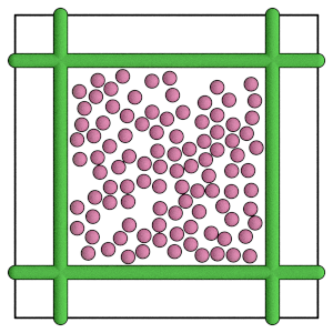
Conclusion

This section demonstrates how to apply a force between wall geometries and particles during Molecular Dynamics simulations. The next section shows how to run the same simulation with hard particle Monte Carlo.